The problem of overfitting in machine learning algorithms

By now in my First approach to machine learning series I have written about two of the most famous building block algorithms: linear regression and logistic regression. We know they can be very powerful yet, as the number of features increase, they might both suffer of a common problem: overfitting. Let's take a closer look at it.

Overfitting: what is it about?

Overfitting, or high variance, happens when your hypothesis function [texi]h_\theta(x)[texi] tries too hard to fit the training set. The result is that the learned hypothesis function will work great with the training set you initially provided, but will fail to generalize new examples.

Your algorithm can also face the opposite problem, called called underfitting, or high bias: the hypothesis function doesn't fit much well the data you have provided in the training stage.

1. Examples of underfitting and overfitting in linear regression.

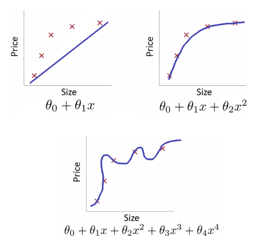
Picture 1. above depicts two cases of wrong fitting during a linear regression task (the famous house prediction problem we saw in earlier articles). The top-left plot shows underfitting: the hypothesis function is a linear one, which doesn't fit so well the data. The top-right plot shows a quadratic function: visually it seems to generalize data pretty well. This is the way to go. The last plot at the bottom shows instead an example of overfitting, where the curve does touch all the points in the training examples (which is good), but with too much juggling. Such hypothesis function will struggle to predict new prices if fed with new examples outside the training set.

Logistic regression too can suffer from bad fitting. As in linear regression, the problem here lies in the hypothesis function trying to separate too much the training examples.

2. Examples of underfitting and overfitting in logistic regression.

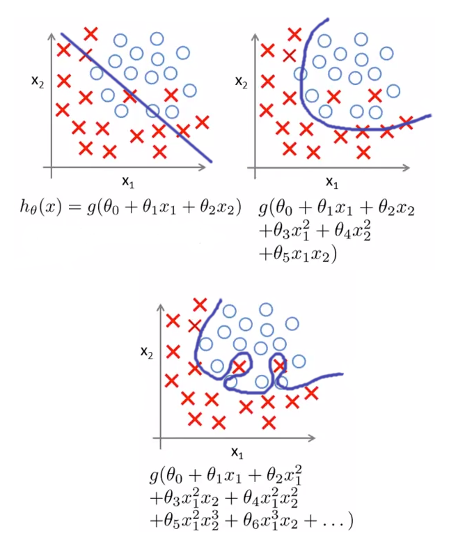
The top-left plot in image 2. above shows an underfitting logistic regression hypothesis function. The data is not well separated by such simplistic linear function. Conversely, a slightly more complex function in the top-right figure does a good job in fitting the data. The third bottom plot shows overfitting: the hypothesis function tries to hard to separate elements in the training set by producing a highly twisted decision boundary.

How to limit overfitting

In a perfect universe your machine learning problem deals with low-dimensional data, that is few input parameters. This is something we saw earlier in our house price prediction examples: we only had "size" and "price" parameters back then, producing a straightforward 2-D plot. Finding overfitting is easy here: just plot the hypothesis function and adjust the formula accordingly.

However this solution is impractical when your learning problem deals with lots (hundreds) of features. There are two main options here:

• Reduce the number of features — you manually look through the list of features and decide what are the most important ones to keep. A class of algorithms called model selection algorithms automatically select the most relevant features: we will take a look at it in the future chapters. Either way, reducing the number of features fixes the overfitting problem, but it is a less than ideal solution. The disadvantage is that you are throwing away precious information you have about the problem.

• Regularization — you keep all the features, but reduce the magnitude (i.e. the value) of each parameter [texi]\theta_j[texi]. This method works well when you have a lot of features, each of which contributes a bit to predicting the output [texi]y[texi]. Let's take a look at this technique and apply it to the learning algorithms we already know, in order to keep overfitting at bay.

A regularized cost function

Say we have two hypothesis functions from the same data set (take a look at picture 1. as a reference): the first one is [texi]h_\theta(x) = \theta_0 + \theta_1 x + \theta_2 x^{2}[texi] and it works well; the second one is [texi]h_\theta(x) = \theta_0 + \theta_1 x + \theta_2 x^2 + \theta_3 x^3 + \theta_4 x^4[texi] and it suffers from overfitting. The training data is the same, so the second function must have something wrong in its formula. It turns out that those two parameters [texi]\theta_3[texi] and [texi]\theta_4[texi] contribute too much to the curliness of the function.

The core idea: penalize those additional parameters and make them very small, so that they will contribute less, or even don't contribute at all to the function shape. If we set [texi]\theta_3 \approx 0[texi] and [texi]\theta_4 \approx 0[texi] (in words: set them to very small values, next to zero) we would basically end up with the first function, which fits well the data.

A real implementation of a regularized cost function pushes the idea even further: all parameters values are reduced by some amount, producing a somehow simpler, or smoother hypothesis function (and it can be proven mathematically).

For example, say we are working with the usual linear regression problem of house price prediction. We have:

• [texi]100[texi] features: [texi]x_1, x_2, \cdots, x_{100}[texi] (size, number of floors, ...) that produce...
• [texi]100[texi] parameters: [texi]\theta_0, \theta_1, \cdots, \theta_{100}[texi]

Of course is nearly impossible to know which parameter contributes more or less to the overfitting issue. So in regularization we modify the cost function to shrink all parameters by some amount.

The original cost function for linear regression is:

[tex] J(\theta) = \frac{1}{2m} \sum_{i=1}^{m} (h_\theta(x^{(i)}) - y^{(i)})^2 [tex]

The regularized version adds an extra term, called regularization term that shrinks all the parameters:

[tex] J_{reg}(\theta) = \frac{1}{2m} \bigg[\sum_{i=1}^{m} (h_\theta(x^{(i)}) - y^{(i)})^2 + \lambda \sum_{j=1}^{m} \theta_j^2\bigg] [tex]

The lambda symbol ([texi]\lambda[texi]) is called the regularization parameter and it is responsible for a trade-off between fitting the training set well and keeping each parameter small. By convention the first parameter [texi]\theta_0[texi] is left unprocessed, as the loop in the regularization term starts from 1 (i.e. [texi]j=1[texi]).

The regularization parameter must be chosen carefully. If its too large, it will crush all the parameters except the first one, ending up with a hypothesis function like [texi]h_\theta(x) = \theta_0[texi] where all other [texi]\theta[texi]s are next to zero. Such function is a simple horizontal line, which of course doesn't fit well the data (and suffers from underfitting).

There are some advanced techniques to find the regularization parameter automatically. We will take a look at some of those in future episodes. For now, let's see how to apply the regularization process to linear regression and logistic regression algorithms.

Regularized linear regression

In order to build a regularized linear regression, we have to tweak the gradient descent algorithm. The original one, outlined in a previous chapter looked like this:

[tex] \begin{align*} & \text{repeat until convergence:} \; \lbrace \newline \; & \theta_0 := \theta_0 - \alpha \frac{1}{m} \sum\limits_{i=1}^{m} (h_\theta(x^{(i)}) - y^{(i)}) \cdot x_0^{(i)} \newline \; & \cdots \newline \; & \theta_j := \theta_j - \alpha \frac{1}{m} \sum\limits_{i=1}^{m} (h_\theta(x^{(i)}) - y^{(i)}) \cdot x_j^{(i)} & \newline \rbrace \end{align*} [tex]

Nothing new, right? The derivative at this point has been already computed and we plugged it into the formula. In order to upgrade this into a regularized algorithm, we have to figure out the derivative for the new regularized cost function seen above.

As always I will lift you the burden of the manual computation. This is how it looks like:

[tex] \frac{\partial}{\partial \theta_j} J_{reg}(\theta) = \frac{1}{m} \sum\limits_{i=1}^{m} (h_\theta(x^{(i)}) - y^{(i)}) \cdot x_j^{(i)} + \frac{\lambda}{m}\theta_j [tex]

And now we are ready to plug it into the gradient descent algorithm. Note how the first [texi]\theta_0[texi] is left unprocessed, as we said earlier:

[tex] \begin{align*} & \text{repeat until convergence:} \; \lbrace \newline \; & \theta_0 := \theta_0 - \alpha \frac{1}{m} \sum\limits_{i=1}^{m} (h_\theta(x^{(i)}) - y^{(i)}) \cdot x_0^{(i)} \newline \; & \cdots \newline \; & \theta_j := \theta_j - \alpha \frac{1}{m} \sum\limits_{i=1}^{m} (h_\theta(x^{(i)}) - y^{(i)}) \cdot x_j^{(i)} + \frac{\lambda}{m}\theta_j & \newline \rbrace \end{align*} [tex]

We can do even better. Let's group all the terms together that depends on [texi]\theta_j[texi] (and [texi]\theta_0[texi] left untouched as always):

[tex] \begin{align*} & \text{repeat until convergence:} \; \lbrace \newline \; & \theta_0 := \theta_0 - \alpha \frac{1}{m} \sum\limits_{i=1}^{m} (h_\theta(x^{(i)}) - y^{(i)}) \cdot x_0^{(i)} \newline \; & \cdots \newline \; & \theta_j := \theta_j(1 - \alpha \frac{\lambda}{m}) - \alpha \frac{1}{m} \sum\limits_{i=1}^{m} (h_\theta(x^{(i)}) - y^{(i)}) \cdot x_j^{(i)} & \newline \rbrace \end{align*} [tex]

I have simply rearranged things around in each [texi]\theta_j[texi] update, except for [texi]\theta_0[texi]. This alternate way of writing shows the regularization in action: as you may see, the term [texi](1 - \alpha \frac{\lambda}{m})[texi] multiplies [texi]\theta_j[texi] and it's responsible for its shrinkage. The rest of the equation is the same as before the whole regularization thing.

Regularized logistic regression

As seen in the previous article, the gradient descent algorithm for logistic regression looks identical to the linear regression one. So the good news is that we can apply the very same regularization trick as we did above in order to shrink the [texi]\theta[texi]s parameters.

The original, non-regularized cost function for logistic regression looks like:

[tex] J(\theta) = - \dfrac{1}{m} \left[\sum_{i=1}^{m} y^{(i)} \log(h_\theta(x^{(i)})) + (1 - y^{(i)}) \log(1-h_\theta(x^{(i)}))\right] [tex]

As we did in the regularized linear regression, we have to add the regularization term that shrinks all the parameters. It is slightly different here:

[tex] J_{reg}(\theta) = - \dfrac{1}{m} \left[\sum_{i=1}^{m} y^{(i)} \log(h_\theta(x^{(i)})) + (1 - y^{(i)}) \log(1-h_\theta(x^{(i)}))\right] + \frac{\lambda}{2m} \sum_{j=1}^{n} \theta_j^2 [tex]

What is the derivative of this baby?

[tex] \frac{\partial}{\partial \theta_j} J_{reg}(\theta) = \theta_j - \alpha \left[\dfrac{1}{m} \sum_{i=1}^{m} (h_\theta(x^{(i)}) - y^{(i)})x_j^{(i)} + \frac{\lambda}{m}\theta_j\right] [tex]

We are now ready to plug it into the gradient descent algorithm for the logistic regression. As always the first item [texi]\theta_0[texi] is left unprocessed:

[tex] \begin{align*} & \text{repeat until convergence:} \; \lbrace \newline \; & \theta_0 := \theta_0 - \alpha \frac{1}{m} \sum\limits_{i=1}^{m} (h_\theta(x^{(i)}) - y^{(i)}) x_0^{(i)} \newline \; & \cdots \newline \; & \theta_j := \theta_j - \alpha \left[\dfrac{1}{m} \sum_{i=1}^{m} (h_\theta(x^{(i)}) - y^{(i)})x_j^{(i)} + \frac{\lambda}{m}\theta_j\right] & \newline \rbrace \end{align*} [tex]

Sources

Machine Learning @ Coursera - The Problem of Overfitting
Machine Learning @ Coursera - Cost Function
Machine Learning @ Coursera - Regularized Linear Regression
Machine Learning @ Coursera - Regularized Logistic Regression)